Topological Map Dataset

Overview

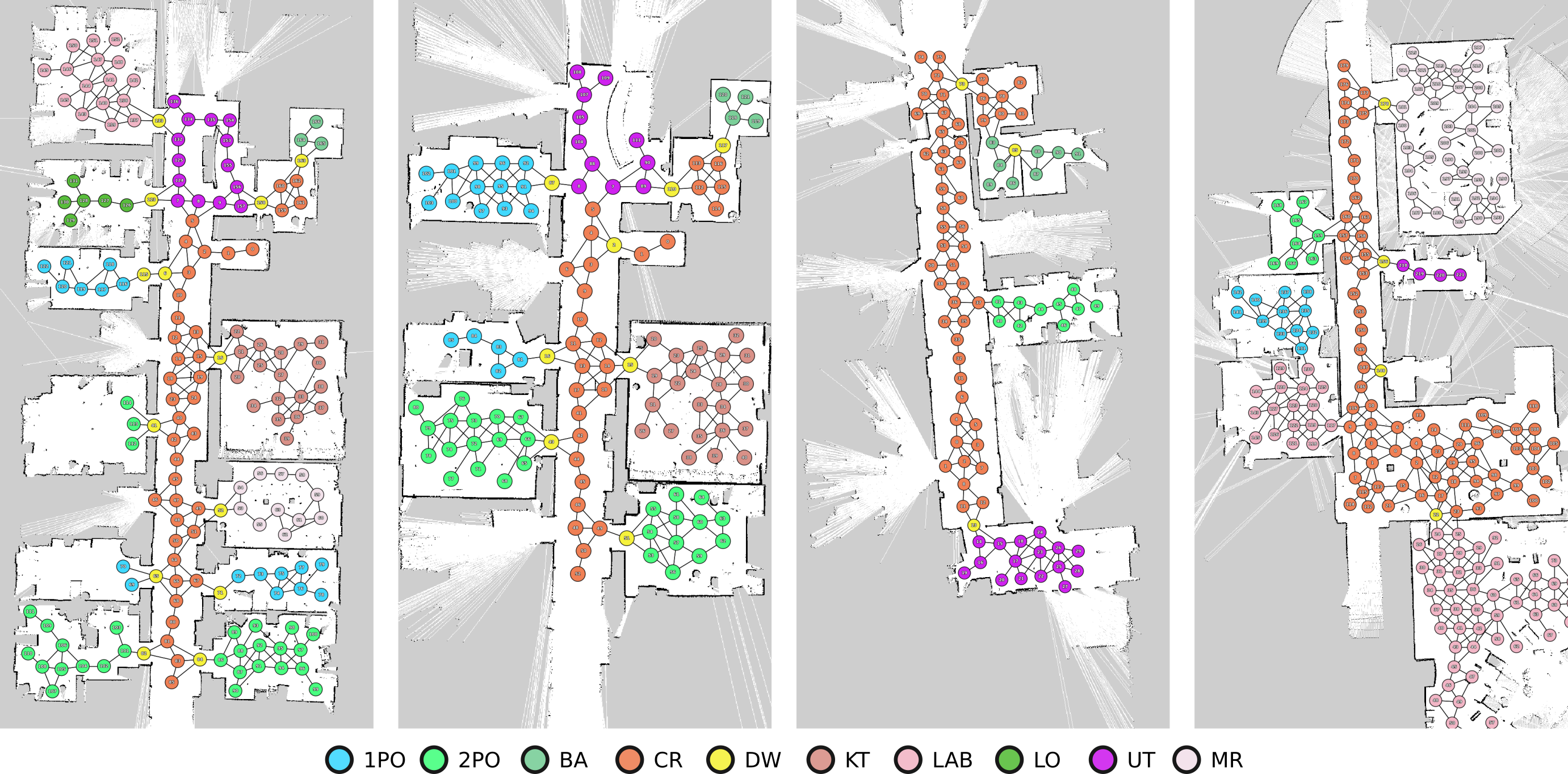
Examples of topological maps

The COLD-TopoMaps Dataset consists of topological maps collected as the robot explores the environment. Each topological map is an undirected graph (also called "topological graph"), where vertices are places that the robot could access, and edges indicate navigability. Each place is annotated by a semantic place category, such as corridor, kitchen, or doorway. As shown in the video below (click to redirect to YouTube), our algorithm for constructing topological graph results in relatively dense graphs, which can be used for planning actions. This dataset aims at providing a benchmark and training data for learning structured prediction models over graphs of uncertain size and structure. It can also be used for research on topological mapping, robot planning etc.

Details

Format

In each sequence, there are four files: nodes.dat, rooms.dat, topo_map.png, and topo_map.yaml. You will most likely only need to process nodes.dat and rooms.dat, while topo_map.png is only used for visualization, and topo_map.yaml is a raw ROS message that records the topological map as it was created. We will describe each separately as follows.

nodes.dat A CSV file where each row is the data for a certain node on the topological map, and each column is an attribute of the node. The column values (and types) are below (... means you don't need to worry about this data attribute):

node ID	placeholder	X (m)	Y (m)	...	...	...	...	...	...	label	...	(views)
int	boolean	float	float							string		(see below)

Each place has 8 views (as shown in the figure below). For every edge connected to the node through a view, there are three entries of data in the row for this node:

neighbor node ID	affordance	view number
int	float	int

If neighbor node ID is -1 for a view number, then this view has no connected edge. If we think of a node as a disk, then the view numbers correspond to regions as annotated in the following illustration.

Note that the order of these 3-tuple columns is arbitrary (i.e. the tuple for view 5 may appear before or after view 7). You most likely don't need to consider this fact. Also, note that placeholder refers to a place where the robot can access but has not explored.

rooms.dat A CSV file where each row contains two columns, the node ID, and the ROOM_ID for that node. ROOM_ID has the same format as in COLD-PlaceScans, which has the pattern {FLOOR_LEVEL}-{ROOM_CATEGORY}-{CATEGORY_INSTANCE_ID}. For example, 4-1PO-2 refers to a room on floor 4, with category 1PO (one-person office) and it is the second 1PO room instance on floor 4. Refer to the table in COLD-PlaceScans about the list of {ROOM_CATEGORY} values.

topo_map.png A PNG file of the visualization of the topological map on top of the SLAM map. Examples are shown at the top of this page. The node ID of a node is shown on top of that node in white bold font. Colors indicate place category, and the mapping is specified in the figure at top.

topo_map.yaml A file generated as a result of running our topological graph construction ROS node, which is an online method for constructing topological graphs and publishes a message of the generated map. This file represents the last message that the ROS node sent before the robot stopped the maneuver. You can think of nodes.dat as the result of processing topo_map.yaml into an easier-to-work-with format. This explained in more detail next.

Acquisition procedure

Here, we describe how our method of topological graph construction works. The method requires a stream of localized robot poses on an occupancy grid map (generated by SLAM). In the ROS framework, robot poses should be published to a topic, while the occupancy grid map should be published to another (using map_server), which means the method should work on-line as the robot explores a new environment. Nevertheless, for our data collection process, we obtained the SLAM map before building the topological graphs. In addition, we used canonical robot poses in the COLD-Meta, which are obtained from AMCL (Adaptive Monte Carlo Localization).

Our algorithm samples, from the occupancy grid map, locations of places (i.e. nodes) based on a probabilistic formulation. This method was proposed in [1] and is also explained in detail in [2]. We briefly summarizes it here [2]:

The topological graph is assembled incrementally based on dynamically expanding 2D occupancy map. The 2D map is built from laser range data captured by the robot using ... (GMapping [3])... approach ... Given the current state of the 2D map, placeholders are added at neighboring, reachable, but unexplored locations and connected to already existing places. Then, once the robot performs an exploration action and navigates to a placeholder, it is converted into a place with local evidence attached.

For mathematical details, please refer to [1] and [2].

Class mapping

Since some categories only appear in one of the three buildings, in our previous use cases of this dataset, we mapped these categories to more common, canonical categories. Here are some mapping setups that we recommend; we map a string label to an integer, then map from that integer to a canonical string label. Note that classes that are not included in FW (forward) are considered unknown (i.e. of class UN)

4-class

{
    'FW': {
        'DW': 0,
        'CR': 1,
        '1PO': 2,
        '2PO': 3,
        'MPO': 3,
        'PRO': 3,
        'UN': 4
    },
    'BW': {
        0: 'DW',
        1: 'CR',
        2: '1PO',
        3: '2PO',
        4: 'UN'
    }
}

10-class

{
    'FW': {
        'OC': -1,
        'DW': 0,   #               (DW)
        'CR': 1,   # corridor      (CR)
        'AT': 1,   # anteroom      (CR)
        'ST': 1,   # stairs        (CR)
        'EV': 1,   # elevator      (CR)
        '1PO': 2,  #               (1PO)
        '2PO': 3,  #               (2PO)
        'PRO': 3,  #               (2PO)
        'MPO': 4,  #               (LO)
        'LO': 4,   # large office  (LO)
        'LAB': 5,  # --lab---LAB-------
        'RL': 5,   # robot lab     (LAB)
        'LR': 5,   # living room   (LAB)
        'TR': 5,   # terminal room (LAB)
        'BA': 6,   # bathroom      (BA)
        'KT': 7,   # kitchen       (KT)
        'MR': 8,   # meeting room  (MR)
        'LMR': 8,  # lg meeting rm (MR)
        'CF': 8,   # conference rm (MR)
        'UT': 9,   # --utility-UT-----
        'WS': 9,   # workshop      (UT)
        'PT': 9,   # printer room  (UT)
        'PA': 9,   # -same as PT-  (UT)
        'UN': 10
    },
    'BW': {
        0: 'DW',
        1: 'CR',
        2: '1PO',
        3: '2PO',
        4: 'LO',
        5: 'LAB',
        6: 'BA',
        7: 'KT',
        8: 'MR',
        9: 'UT',  # utility
        10: 'UN'
    },
}

Download

The COLD-TopoMaps dataset is now available in the GraphSPN repository. Clone this repository, and the dataset is under graphspn/experiments/datasets/cold-topomaps.

Usage

Parsing nodes.dat and rooms.dat to construct a topological map could be a tedious programming problem. Here we provide two Python classes, TopoMapDataset (here) and TopologicalMap (here), which hopefully help with this process. Here is an example of using the above two classes:

# Visualize topological maps

dataset = TopoMapDataset(PATH_TO_TOPO_MAP_DB_ROOT)
dataset.load("Stockholm", skip_unknown=True, skip_placeholders=False, single_component=False)
topo_maps = dataset.get_topo_maps(db_name="Stockholm", amount=10, seq_id=seq_id)
for seq_id in topo_maps:
    topo_map = topo_maps[seq_id]
    topo_map.visualize(plt.gca(), GROUNDTRUTH_MAP_YAML_FILE), show_nids=True)
    plt.savefig('%s.png' % seq_id)
    plt.clf()
    plt.close()

Regarding GROUNDTRUTH_MAP_YAML_FILE, please refer to the description of groundtruth data in COLD-Meta.

Citation

@inproceedings{zheng2018aaai,
  author =       {Zheng, Kaiyu and Pronobis, Andrzej and Rao, Rajesh P. N.},
  title =        {Learning {G}raph-{S}tructured {S}um-{P}roduct {N}etworks for Probabilistic Semantic Maps},
  booktitle =    {Proceedings of the 32nd AAAI Conference on Artificial Intelligence (AAAI)},
  year =         2018,
  address =      {New Orleans, LA, USA},
  month =        feb,
  archivePrefix = {arXiv},
  primaryClass = {cs.LG},
  eprint =       {1709.08274}
}

References

[1] A. Pronobis, F. Riccio, R. P. N. Rao, Deep Spatial Affordance Hierarchy: Spatial Knowledge Representation for Planning in Large-scale Environments
[2] K. Zheng, A. Pronobis and R. P. N. Rao, "Learning {G}raph-{S}tructured {S}um-{P}roduct {N}etworks for Probabilistic Semantic Maps,", Proceedings of the 32nd AAAI Conference on Artificial Intelligence (AAAI), 2018.
[3] https://openslam-org.github.io/gmapping.html<b