COLD-Metadata

Overview

The COLD-Meta Dataset, as the name suggests, is a dataset of the metadata produced by robot sensors as well as basic information about the robot operation. In particular, it contains:

• Odometry (20 Hz). odometry.dat
• Laser range data (10 Hz). scans.dat
• Annotations by timestamp (30 Hz). labels.dat
• Annotations by data type (frequency varies). labels_{datatype.dat}
• Localized robot poses (30 Hz). canonical_poses.dat
  • Visualization of localized robot path. canonical_path.png, canonical_path.svg
• SLAM poses (30 Hz). poses.dat
  • Visualization of SLAM path. path.png, path.svg
  • This is used as a validation of the quality of SLAM, which depends on the quality of odometry and laser range data.
• SLAM map. map.png, map.pgm, map.yaml
• ROS bag file. data.bag
  • metadata for this bag file is also included. data.json
• Groundtruth, including the canonical maps for each floor and room annotations.
  • Included in the groundtruth directory.
  • Room annotations are specified in labels.json and visualized in labels.png.

It is an expensive and significant effort to collect a large and organized robotic dataset as such that includes metadata of numerous modalities of information. We hope that our effort is paid off by advancing research of indoor mobile robots and beyond. This metadata dataset is a good resource for fundamental robotics problems such as SLAM, localization and navigation. By design, before you could download COLD-PlaceScans dataset and COLD-Images dataset, you would need to first download the COLD-Meta dataset, which contains shell scripts that download the other datasets for you automatically.

Details

Format

Odometry The 20 Hz odometry is stored in odometry.dat, a CSV file with the following format.

id	timestamp	x (m)	y (m)	th (rad)
int	float	float	float	float

The timestamp is of Unix epoch format, with 6 digits after the decimal (i.e. 10^-6 s).

Laser-range The 10 Hz laser range data is stored in scans.dat, a CSV file with the following format.

id	timestamp	n_beams	readings ...	angle_min (rad)	angle_increment (rad)	range_max (m)	range_min (m)
int	float	int	floats	float	float	float	float

The timestamp is of Unix epoch format, with 6 digits after the decimal (i.e. 10^-6 s). The n_beams is the number of laser beams shooting from the sensor, which determines the number of entries in readings..., a list of floats that indicate the reading for each beam. The angle_min, angle_increment, range_min, range_max are defined in the sensor_msgs/LaserScan message of ROS. Note that angle_max can be computed from other entries as follows:

angle_max = n_beams * angle_increment + angle_min

Annotations We provide semantic annotation of the robot localization in two ways: by timestamp, and by data type. We describe each as follows.

By timestamp In the CSV file labels.dat, there is a 30 Hz stream of room labels, where each row has the following format.

timestamp	floor	label	category_instance_id
float	int	string	int

The timestamp is of Unix epoch format, with 6 digits after the decimal (i.e. 10^-6 s). The label is an abbreviation of room category (e.g. CR for corridor). These labels are decided based on the groundtruth information of the floor plan, as well as the localization provided by AMCL (see details in the next section). The complete list of labels is provided in COLD-PlaceScans. The category_instance_id is used to differentiate rooms of the same category on the same floor.

Note that room_id (defined as ROOM_ID in COLD-PlaceScans) is constructued as {floor}-{label}-{category_instance_id} (e.g. 4-DW-1).

By data type There are several CSV files named labels_{datatype}.dat, where datatype is a data modality (e.g. place scans, prosilica camera, omnidirectional camera, see COLD-Images). The format of each row in these files is as follows.

id	timestamp	room_id
int	float	string

The timestamp is of Unix epoch format, with precision depending on the timestamp of the data for the datatype. For each data point with datatype (e.g. an image of omnidirectional camera), we match it with the closest room_id by timestamp based on labels.dat.

Note: For some datatype of some sequences, some data points have timestamps is too early (or too late) compared to the timestamps of labels. For example, sequence floor4_cloudy_a1, proscilica_left, the first data point has timestamp of 1205845874.784, but the first label in labels.dat (created by annotating each pose), has timestamp 1205845877.363672, a difference of 3 seconds

Poses For each sequence of metadata, there are two pose files, canonical_poses.dat and poses.dat. The former is more useful; it contains poses produced by AMCL localization on the canonical map (i.e. groundtruth map), using the laser-range data and odometry of this sequence. The latter contains poses of SLAM using also the laser-range data and odometry of this sequence. Since different sequences result in different SLAM maps, the SLAM poses of sequences on the same floor are not with respect to the same origin, while the AMCL poses do. The format of these two dat files are as follows.

timestamp	x (m)	y (m)	th (rad)
float	float	float	float

The timestamp is of Unix epoch format, with 6 digits after the decimal (i.e. 10^-6 s).

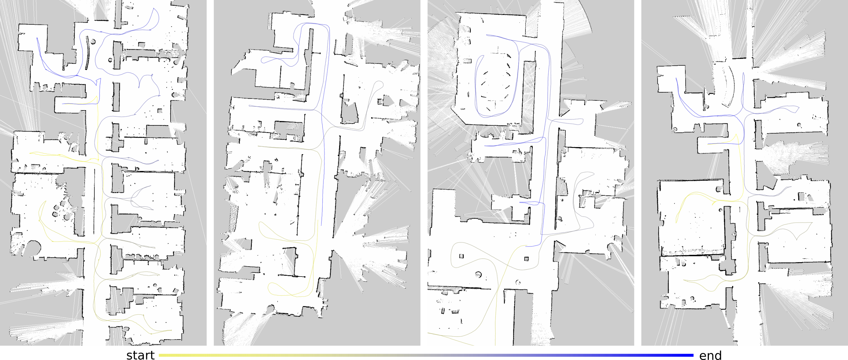
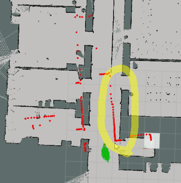
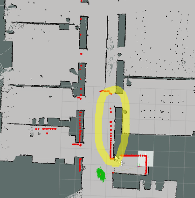
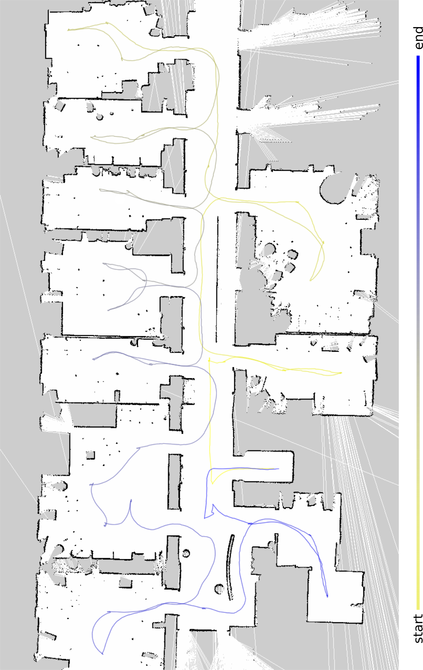
We also provide visualization of both poses, in canonical_paths.(png|svg) and paths.(png|svg), for AMCL poses and SLAM poses, respectively. Examples of canonical path visualizations are provided below. See the bottom of this page for a zoomed-in version of the first visualization.

Examples of canonical path visualizations

SLAM map We ran SLAM for each sequence, given the odometry and laser range observations, using the ROS gmapping package. The results are provided in map.png, map.pgm and map.yaml. Note that oth map.png and map.pgm contain only three colors: white (free space), black (obstacle) and grey (unknown). For each floor, we select a good-quality SLAM map as the canonical map to represent the floor, and this map is collected in the groundtruth.

ROS bags For every sequence, we also include a bag file, created by the rosbag package. A bag file is a standard format in ROS for storing ROS message data which allows playback for both online and offline use. Below is a screenshot of rqt_bag reading a bag file.

As shown, there are three topics in the bag file: mobile_base/odometry which publishes nav_msgs/Odometry messages, scan which publishes sensor_msgs/LaserScan messages, and tf which publishes the tf/tfMessage messages, that is, the tf transform from odom to base_footprint (see REP 120). The data.json file contains metadata for this ROS bag file:

{
    "init_posit": list of floats,  # [x,y,z] of initial position
    "init_orien": list of floats,  # [x,y,z,w] of initial orientation
    "seq_id": string,  # sequence id, e.g. floor4_cloudy_a1
    "start_time": float,  # timestamp of the start time of messages
    "end_time": float     # timestamp of the end time of messages
}

Note that the information in scans.dat are not sufficient to fill all the fields in the sensor_msgs/LaserScan message, such as scan_time. To resolve this issue, we obtained configurations of the laser scanner that we have used for data collection. We used SICK LMS 200 for Stockholm (refer to this issue),

{   
    "range_min": 0.0,
    "range_max": 81.0,
    "angle_min": -1.57079637051,
    "angle_max": 1.57079637051,
    "angle_increment": 0.0174532923847,
    "time_increment": 3.70370362361e-05,
    "scan_time": 0.0133333336562
}

And we used SICK LMS 291 for Freiburg and Saarbrücken

{   
    "range_min": 0.0,
    "range_max": 81.0,
    "angle_min": -1.57079637051,
    "angle_max": 1.57079637051,
    "angle_increment": 0.00872664619235,
    "time_increment": 7.40740724722e-05,
    "scan_time": 0.0133333336562
}

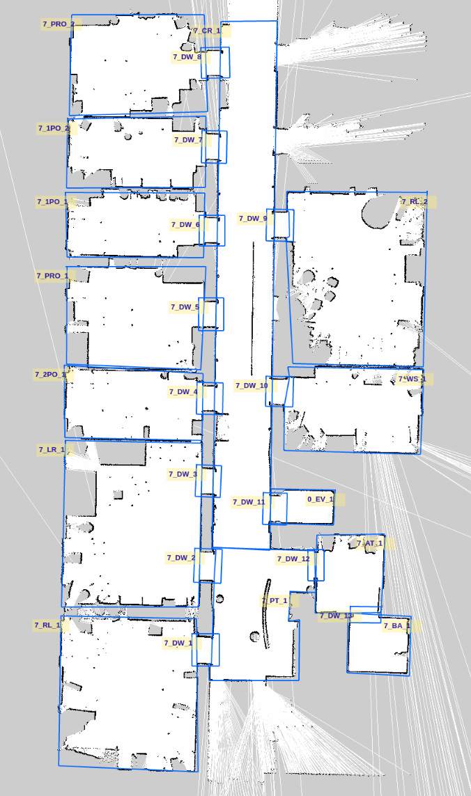
Groundtruth In each metadata repository that you download (e.g. cold-stockholm), there is a groundtruth directory, which contains directories for the groundtruth information for each floor (e.g. floor4). In the directory for each floor, there are 5 files. Among them, the map.png, map.pgm, map.yaml are canonical SLAM maps selected from the sequences for that floor. The labels.png, labels.json. are information regarding room annotations. Here, labels.json is a JSON specification of the rooms, with format:

{
    "rooms":
        "room_N":
            {
                "objects": {},  # this information is not yet acquired
                "unique_id": {floor}_{label}_{category_instance_id},  # room id
                "outline":  # List of edges of the room outline
                    [
                        [x, y]    # with respect to gmapping coordinates of the map
                    ]
...

The labels.png is the visualization of the label specification. See the bottom of this page for an example. The annotation process is created by this JavaScript tool. To determine if a gmapping point is within a room specified as above, we can use the code (in Python) here:

Acquisition Procedure

Among all metadata files for a sequence, only odometry.dat and scans.dat are raw data; everything else is produced based on top of them. The pipeline of our data acquisition procedure is illustrated in the diagram below:

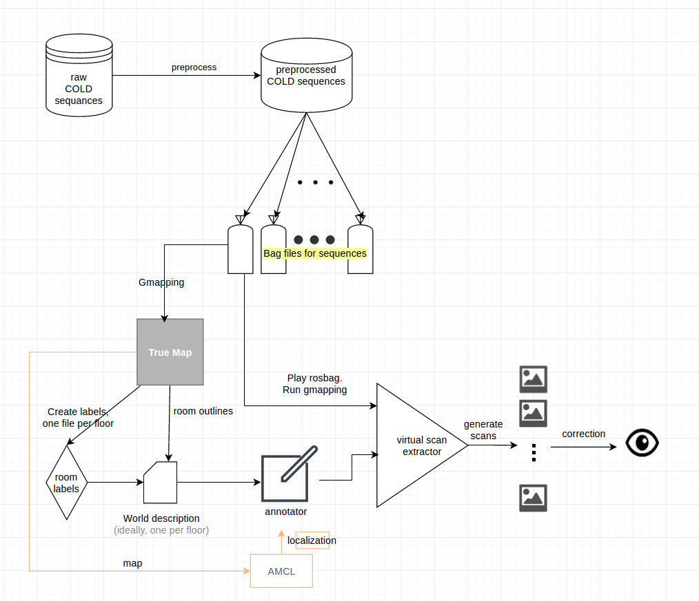
This procedure can be summarized into 5 steps:

1. Preprocess raw COLD data file.
2. Generate bag files from preprocessed COLD data.
3. Generate SLAM maps.
4. Select canonical maps (i.e. true maps), one per floor, and draw outlines using the webtool, and generate world descriptions (i.e. labels.json).
5. Generate place scans (or "virtual scans" as termed in the illustration).

Robot platform

To be completed.

Localization

We estimate robot poses using AMCL, the ROS implementation of the popular Monte-Carlo Localization (MCL) algorithm proposed by Fox et al. (1999) [1]. This algorithm takes as input the laser range observations, odometry data, as well as a canonical 2D occupancy grid map. For each group of sequences that are collected on the same floor, we use GMapping, described by Grisetti et al. (2007) [2], to generate a SLAM map used as the canonical map for that floor. Then, by taking streams of laser range observations and odometry data, AMCL maintains internally the motion and measurement models, and uses them to iteratively resample the position and orientation of a pool of particles.

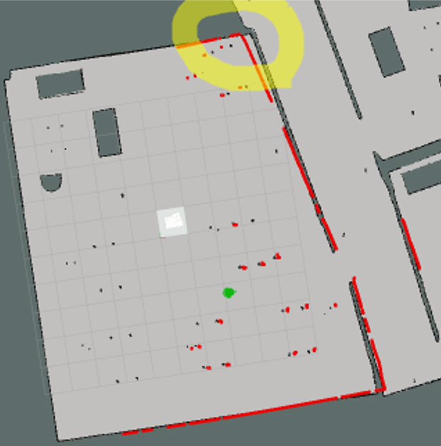
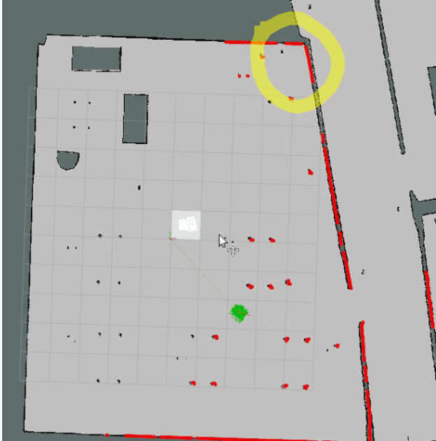
To guarantee optimal localization performance, we made sure that the laser scan messages contain the correct fields for the laser scanner product used (see the parameters for SICK LMS 200 and LMS 291 above). Additionally, we fine tuned the parameters for both the motion and measurement model, so that (1) the visualization of the laser range readings consistently matches with the walls and large obstacles in the environment tightly, and (2) the particles are relatively condensed.

when LaserScan fields are not correct	when LaserScan fields are correct	default measurement model parameters	after tuning

Here are the parameters for measurement model and motion model that we used for AMCL. For measurement model, we increased laser_z_hit and laser_sigma_hit to incorporate higher measurement noise. For motion model, we tuned the parameter so that the algorithm assumes there is low noise in odometry.

# Measurement model
{
    "laser_z_hit": 0.9,
    "laser_sigma_hit": 0.1,
    "laser_z_rand" :0.5,
    "laser_likelihood_max_dist": 4.0
}

# Motion model
{   
    "kld_err": 0.01,
    "kld_z": 0.99,
    "odom_alpha1": 0.005,
    "odom_alpha2": 0.005,
    "odom_alpha3": 0.005,
    "odom_alpha4": 0.005
}

We use the ROS tf package to maintain transformations of the robot’s position with respect to the map origin, and between the laser scanner and the robot center (more on this next). This allows us to record the localized pose at a high frequency of 30Hz. We visualize the robot poses on the canonical map for each sequence in the database, as the example in figure 2 shows

Another important issue that affects the quality of localization is the position of the laser scanner in the tf tree, namely, the transition between laser_link and base_footprint. If this value is off, the localization is likely shifted and may be less stable. For our robot used in Stockholm, the laser scanner was roughly placed 27 cm in the +x direction from the center; Thus we published a tf transform from laser_link to base_footprint with translation (0.27, 0.0, 0.0). For our robots used in Freiburg and Saarbrücken, the laser scanner was placed around the center of the robot, thus the translation was (0.27, 0.0, 0.0).

Download

The metadata dataset is actually required to be downloaded prior to downloading any other datasets. You can download the metadata datasets by building from the following repositories:

• cold-stockholm
• cold-freiburg
• cold-saarbruecken

The COLD database is still in preparation and download will be made available soon. Please check back in a few days.

Citation

The paper for COLD database will be available soon.

Visualizations

Zoomed-in view of an example path visualization

Zoomed-in view of room annotations

References

[1] D. Fox, W. Burgard, F. Dellaert, and S. Thrun. "Monte carlo localization: Efficient position estimation for mobile robots," Efficient position estimation for mobile robots. AAAI/IAAI, 1999(343-349), 2-2.
[2] G. Grisetti, S. Cyrill, and W. Burgard. "Improved techniques for grid mapping with rao-blackwellized particle filters." IEEE transactions on Robotics 23.1 (2007): 34.